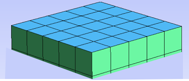
Meshes and domains
Let’s define a mesh:
uint ne1=5, ne2=5, ne3=5;
auto fecX  = FeConnectivity__grid3(n1,n2,n3,1)              // a grid-type connectivity
auto dataX = DataGridFactory::variableN("X",n1+1,n2+1,n3+1) // a grid-type construction of coordinates;
auto X     = vectorN(dataX,3);                              // a grid-type multiple 3D-vector for the coordinates

auto mesh = GmshMesh__get(fecX,X);
mesh.save("cube.msh");
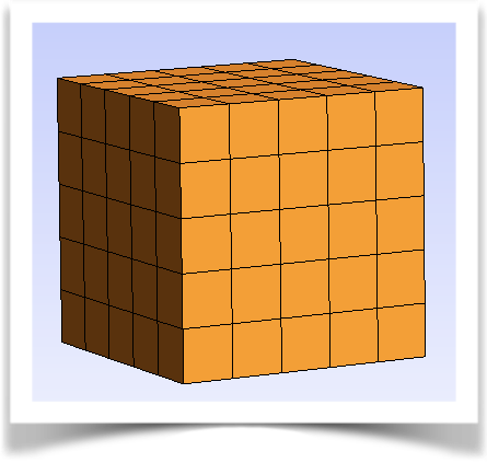
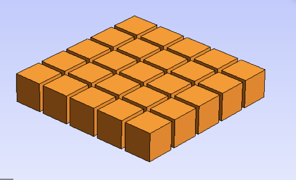
The initial domain stored in file cube.msh
Subdomains
Now, we can build some subdomains by specifying a list of elements. For this, better use a formal function than a list, in order to possibly spare the storage of its values, and considering that this is their more generic definition: a Natural1_FunctionN, that returns a positive index for a positive index entry.
For instance, if the subdomain has all the elements, or a continuous range of them, a simple function can easily define it without storing a list of indices.
uint n = ...;
uint i0 = ...;
auto f_list1 = Natural1_FunctionN__identity(n);     // all values (0,..,n-1)
auto f_list2 = Natural1_FunctionN__linear  (n,i0,2) //  (i0 + 2*i)_{i=0,n-1}

auto fec1 = fecX(f_list); // the corresponding sub-connectivity
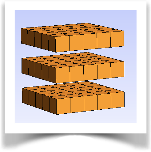
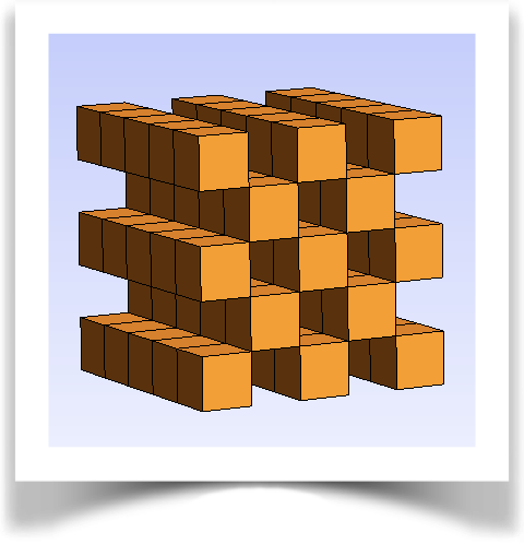
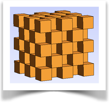
Here are some particular partitions based on the parity of some index.
\(n=3\times n_1\times n_2\) |
\(f:i\rightarrow 2n_1n_2(i÷ (n_1n_2)) + i \%(n_1n_2)\) |
|
\(n=n_1\times ((n_2\times n_3+1)÷2)\) |
\(f:i\rightarrow 2n_1(i ÷ n_1) + i\%n_1\) |
|
\(n=(n_1\times n_2\times n_3)÷2+1\) |
\(f:i\rightarrow 2i\) |
auto nel1 = 3*n1*n2;        auto f_elts1 = Natural1_FunctionN(nel1,[n12=n1*n2](auto i) { return 2*n12*(i/n12) + i%n12; };
auto nel2 = (n1*n2*n3)/2+1; auto f_elts2 = Natural1_FunctionN(nel2,[]         (auto i) { return 2*i;                   };
auto nel1 = (n2*n3+1)/2*n1; auto f_elts3 = Natural1_FunctionN(nel3,[n1]       (auto i) { return 2*n1*(i/n1) + i%n1;    };

// creation of the mesh based on the sub-connectivity
auto mesh = GmshMesh__get(fecX(f_elts1),X);
mesh.save("cube.msh");
Domains
A domain is a connectivity of elements specified only by their vertices and is aimed at defining a parameterization topology, through reference elements and possible identification of neighbours. We can refer to a point by its element index and the local coordinates in it.
A ReferenceDomain has no hole in the numbering of vertices. Two subdomains may have the same ReferenceDomain. On the contrary, RealDomain’s retain the original numbering in order to identify their location in a wider domain.
First of all, we define a domain:
auto domain = ReferenceDomain(fecX);
Sides
An example will help us to see the use of ReferenceSideN.
An example
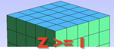
Be a grid mesh with a boundary named « top »:

extracting the sides:
auto sides = sides_extractor<Grid3>("top")(gridX); // ReferenceSideN from a name
and applying it to the connectivity:
auto meshSides    = GmshMesh__get(fecX(sides),X);
auto meshElements = GmshMesh__get(fecX(sides.element_index_function()),X);
yields the following results:
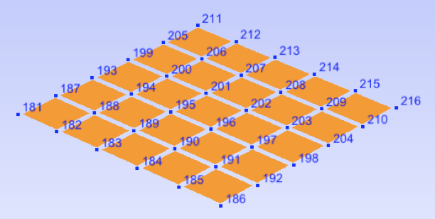
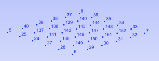
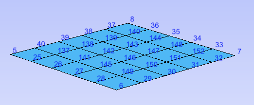
Faces obtained with the ReferenceSideN |
Elements obtained with the ReferenceSideN |
Sides are the sides of reference elements; ReferenceSideN is a list of element indices and the corresponding list of local side indices. A third list can be given: a local numbering index which embeds a mirroring flag and a circular rotation index that specify both the orientation and the starting node for the basis of the local parameterization of coordinates. It is useful for mean and jump computation at the interface of two elements for a discontinous interpolation for instance.
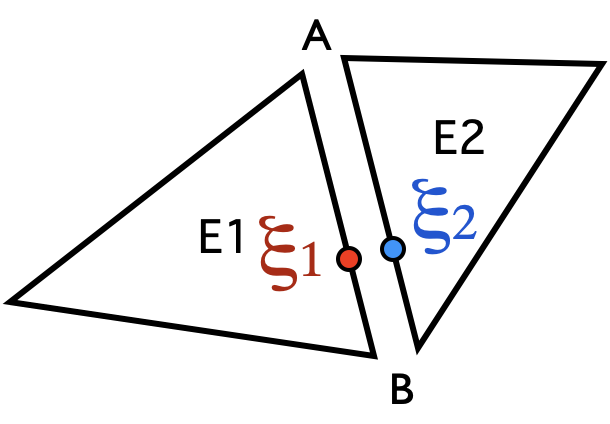
Vis-à-vis correspondance
As the domain element is available, the side element can be oriented: its outward normal can be given. Furthermore, gradients along the normal can be computed, meanwhile computation on the sole finite side element lack derivatives in the missing dimension. Although seldom used because of the classical treatment of Neumann’s boundary conditions, or Lagrange’s multipliers summation to recover the flux through imposed-value boundaries (Dirichlet conditions), it may prove useful for comparisons with numerical integrations of the flux.
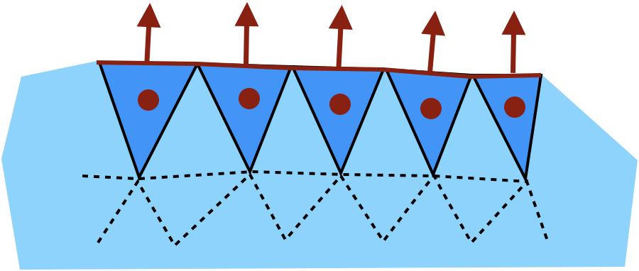
Outward normal
Boundaries
Boundary sides are the sides that appear in only one element.
auto sidesB = boundary_reference_sides(domain); // ReSideN
auto mesh   = GmshMesh__get(fecX(sidesB),X);
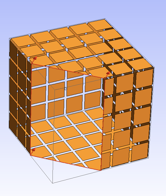
Internal sides
Internal sides are the sides that appear in exactly two elements. There are two separate lists of them: the list of first sides, that of second ones, on the basis of the element number owning the side.
auto sides1 = internal_reference_sides1(domain);
auto mesh   = GmshMesh__get(fecX(sides1),X);
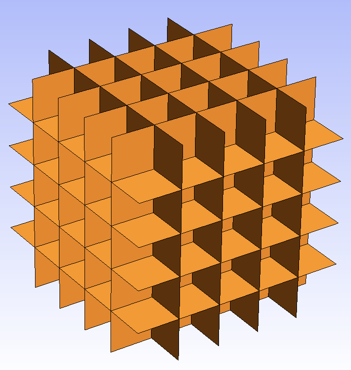
Singular sides
Should a side appear in more than two elements, it would be obtained by the “singular_reference_sides” function: an non empty example will be shown later on the edges.
auto sidesS = singular_reference_sides(domain);
assert(sidesS.domain_size()==0);
Edges as sides of sides (3D)
First of all, we get again the list of first internal sides « sides1 »: 
Boundary edges
Then we can get the sides of the sides, for instance those at the boundary (boundary of the side domain).
auto edgesB    = boundary_reference_sides(domain(sides1));
auto meshEdges = GmshMesh__get(fecX(sides)(edgesB),X);
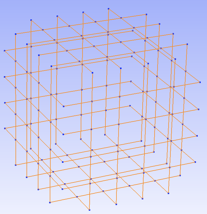
Singular edges
Singular edges are the edges that appear in more than two side elements. As all the internal edges are singular in the internal sides domain, the way to get them is to call “singular_reference_sides” on that domain.
auto edgesS    = singular_reference_sides(domain(sides1));
auto meshEdges = GmshMesh__get(fecX(sides1)(edgesS),X);
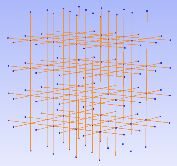
Edges obtained directly
We can get all the edges of a domain. Like sides, a ReferenceEdgeN is a list of edges specified by a list of elements with a list of edge indices and optionnally with an inverting flag to change its orientation.
auto edges = reference_edges(domain); // ReferenceEdgeN
Identifying and extracting sides
How to specify a surface in a mesh?

Many functions are available to extract sides from a mesh, grid or connectivity.
|
|
|
with a name |
with a criterion |
|
|
|
|
with a list of nodes |
with a 2D connectivity |
with a ReferenceSideN |
An example of extraction has been given at the beginning.
